Chapter 3 Impact Analysis
This part of the research uses descriptive statistics to explore and understand terrorist events from various perspectives. This is essential to examine characteristics of attacks and responsible groups over the period of time. Findings and insights from this analysis are eventually helpful to select appropriate data for the statistical modeling part.
3.1 Data preparation
The primary data file globalterrorismdb_0617dist.xlsx used in this research contains over 170,000 terrorist attacks between 1970-2016 (excluding the year 1993). This file can be downloaded by filling up a form on START Consortium’s website.8 This file contains a total of 135 variables categorized by incident ID and date, incident information, attack information, weapon information, target/victim information, perpetrator information, casualties and consequences, and additional information. Out of 135 variables, I have selected a total of 38 variables from each category that are relevant to the research objective. During the data cleaning process, I have made following changes (corrective steps) to original data to make it ready for analysis:
- renaming of some variables (such as
gnametogroup_name,INT_LOGtointl_logistical_attack) to keep the analysis and codes interpretable to a wider audience. - replacing 2.7% NAs in latitude and longitude with country level or closest matching geocodes. Note that most NAs refers to either disputed territories such as Kosovo or countries that no longer exist such as Czechoslovakia.
- 5% NAs in
nkill(number of people killed) and 9% NAs innwound(number of people wounded) variable replaced with 0. GTD reference manual suggests that “Where there is evidence of fatalities, but a figure is not reported or it is too vague to be of use, this field remains blank.” - NAs in regional variables i.e
cityandprovstatereplaced with “unknown”
GTD data is further enriched with country and year wise indicators from World Bank Open Data to get a multi-dimensional view and for modeling part. This data is also open-source and can be accessed through R library WDI.9
List of all the variable with a short description as well as the script to implement the aforementioned steps and to prepare clean dataset can be viewed in Appendix I. Detailed information and explanation about each variable can be found GTD codebook10.
3.2 Global overview
tmp <- df %>% group_by(region, year) %>% summarize(attack_count = n())A quick look at region level number attacks suggests that situation is becoming worst in the Middle East & North Africa followed by South Asia, Sub-Saharan Africa and Southeast Asia where exponential growth in a number of attacks can be observed specifically from years 2010 to 2016. Note that the Y-axis is set free to have closer look at trends.
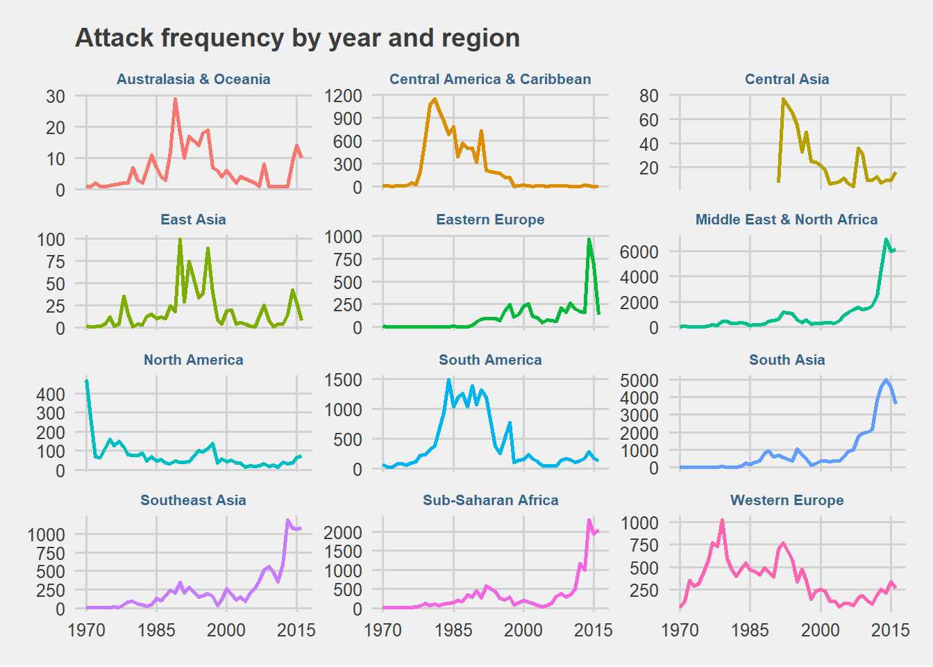
Figure 3.1: Attack frequency by year and region
An interesting observation is in Eastern Europe region where a sudden increase in a number of attacks can be observed during 2014-2015 and then a sudden decrease in 2016. Within the most impacted regions, the nearly similar trend of gradual increase in a number of attacks after 2010 and peak during 2014-2015 is visible. It’s worth mentioning that in June 2014, Islamic State announced the establishment of “Caliphate” while declaring Abu Bakr al-Baghdadi as “leader of Muslims everywhere” and urging other groups to pledge allegiance (Al Jazeera, 2014). Islamic State was at its peak strength during Jan 2014 to Jan 2015 (Ceron et al., 2018).
To understand the attack characteristics, let’s take a look at Frequency of attack type and type of weapon used by terrorist groups.
tmp <- df %>% group_by(attack_type, year) %>% summarise(total_attacks = n()) Figure 3.2: Trend in type of attack in all incidents globally
The heat signatures indicate Bombing/Explosive as one of the frequently used techniques by terrorist groups. Although the pattern in this tactic is visible throughout all the year, while rising during the late 80s and early 90s however it has now increased to nearly 7 times since 2006. A similar pattern (with lower magnitude) can be observed in Armed Assault followed by Hostage Taking and Assassination technique.
tmp <- df %>% group_by(weapon_type, year) %>% summarise(total_attacks = n())Figure 3.3: Trend in type of weapon used in all incidents globally
Upon examining the trends in the type of weapon used in all terrorist incidents globally, it is visible that use of Explosives/Bomb/Dynamites and Firearms is extremely high since 2011 and compared to other weapon types. Use of vehicles as weapon type was relatively low until 2013, however, it was on peak in 2015 with total 34 number of attacks.
Observing trends in target type over the period of time is also a useful way to understand characteristics and ideology among terrorist incidents. As shown in the plot below, the heat signature indicates the top five most frequently attacked target types as Private Citizens & Property followed by Military, Police, Government, and Business.
tmp <- df %>% group_by(target_type, year) %>% summarise(total_attacks = n()) Figure 3.4: Trend in intended targets in all incidents globally
According to GTD codebook, Private Citizens & Property category includes attack on individuals, public in general or attacks in highly populated areas such as markets, commercial streets, busy intersections and pedestrian malls. In a study to investigate when terrorist groups are most or least likely to attack civilians, researcher (Heger, 2010) find a relationship with group’s political motivation and suggests that terror groups pursuing a nationalist agenda are more likely to attack civilians. A relatively lower magnitude trend but with gradual increase in recent years is also visible on Religious Figures/Institution and Terrorist/ Non-state Militia category. The inclusion criteria for Terrorist/ Non-state Militia category refers to terrorists or members of terrorist groups (that are identified in GTD) and broadly defined as informants for terrorist groups excluding former or surrendered terrorists.
3.3 The top 10 most active and violent groups
Findings from exploratory data analysis at region level indicate that the number of attacks have increased significantly from the year 2010 and nearly at the same pace in the Middle East & North Africa, South Asia, Sub-Saharan Africa and Southeast Asia region. Trends in attack type, weapon type and target type over the same period of time (from 2010) suggests that bombings and explosions as a choice of attack type is growing exponentially while the use of explosives & firearms and attacks on civilians is at alarming high level.
This part of the research identifies and examines the top ten most violent and active terrorist groups based on a number of fatalities and number of people injured. GTD codebook suggests that when an attack is a part of multiple attacks, sources sometimes provide a cumulative fatality total for all of the incidents rather than fatality figures for each incident.
In order to determine top ten most active and violent groups based on fatalities and injured while preserving statistical accuracy, first I filter the dataset for the events that took place from 2010 onward and remove the incidents where group name is not known. The new variable impact is the sum of fatalities and the number of people injured. Wherever an attack is observed as a part of multiple attacks, and reported figures are different, I use the figure which is maximum among all the reported figures while ensuring that reported incidents are distinct and grouped by month, year, region and name of the group as shown in the code below:
by_groups <- df %>%
  filter(group_name != "Unknown" & year >= 2010) %>%
  replace_na(list(nkill = 0, nwound = 0)) %>%
  select(group_name, region, year, month, nkill, nwound,
         part_of_multiple_attacks) %>%
  group_by(group_name, region, year, month) %>%
  filter(if_else(part_of_multiple_attacks == 1,
                 nkill == max(nkill) & nwound == max(nwound),
                 nkill == nkill & nwound == nwound)) %>%
  distinct(group_name, region, year, month, nkill, nwound,
           part_of_multiple_attacks) %>%
  mutate(impact = nkill + nwound) %>%
  group_by(group_name) %>%
  summarise(total = sum(impact)) %>%
  arrange(desc(total)) %>%
  head(10)

# create a vector of top 10 groups for further analysis
top10_groups <- as.vector(by_groups$group_name)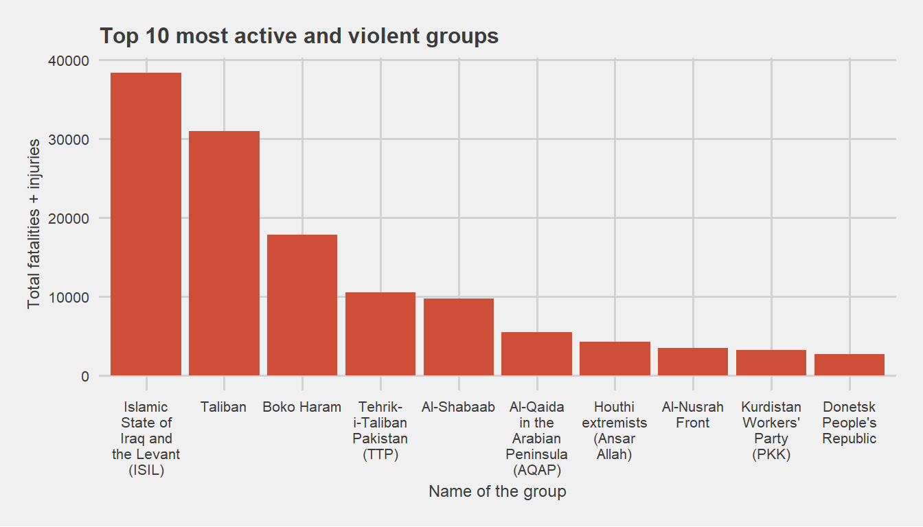
Figure 3.5: Top 10 most active and violent groups
Based on a cumulative number of fatalities and injured people, we can see that ISIL and Taliban, followed by Boko Haram are the most violent groups that are currently active.
To better understand their activity over the period of time, we take a look at attack frequency from each group.
tmp <- df %>%
  filter(group_name %in% top10_groups) %>%
  group_by(group_name, year) %>%
  summarise(total_attacks = n())
Figure 3.6: Attack frequency by Top 10 groups
It’s interesting to see that the majority of this most violent terrorist groups (6 out of 10) were formed after 2006 only. Particularly, a number of attacks from ISIL can be seen increasing rapidly within a shortest period of time (4 years) and a gradual increase in attacks from Taliban (reaching a peak at 1249 in the year 2015).
Attack characteristics for all 10 groups (cumulative) indicate Military as the most frequent target (27.5%) followed by civilians (27.3%). Similarly, Bombing/Explosions and Armed assault as a most frequent attack tactics account for 70.4% of all the attacks as shown in the plots below.
Figure 3.7: Characteristics of top 10 groups
3.4 The major and minor epicenters
The term “Epicenter” used here refers to the geographical location that is impacted by terrorist incidents from top 10 groups as defined. To examine the threat level from this groups by geographic location, I use the cumulative sum of the number of people killed and a number of people wounded as a measurement. Below is the code used to prepare the data for this analysis.
tmp <- df %>%
  filter(group_name %in% top10_groups) %>%
  replace_na(list(nkill = 0, nwound = 0)) %>%
  group_by(group_name, region, year, month) %>%
  filter(if_else(part_of_multiple_attacks == 1,
                 nkill == max(nkill) & nwound == max(nwound),
                 nkill == nkill & nwound == nwound)) %>%
  ungroup() %>%
  distinct(group_name, region, country, year, month, nkill,
           nwound, part_of_multiple_attacks) %>%
  group_by(country, region) %>%
  summarise(attack_count = n(),
            nkill_plus_nwound = sum(nkill + nwound))
# Threat level in four regions
tbl <- tmp %>%
filter(region %in% c("North America", "Eastern Europe",
"Central Asia", "Southeast Asia"))| country | region | attack_count | nkill_plus_nwound |
|---|---|---|---|
| Georgia | Central Asia | 1 | 1 |
| Turkmenistan | Central Asia | 1 | 5 |
| Russia | Eastern Europe | 2 | 6 |
| Ukraine | Eastern Europe | 170 | 2695 |
| United States | North America | 2 | 2 |
| Indonesia | Southeast Asia | 1 | 2 |
| Malaysia | Southeast Asia | 1 | 8 |
| Philippines | Southeast Asia | 6 | 102 |
We can see minor/ negligible threat level across North America and Central Asia region, however, Ukraine turns out to be the major epicenter in Eastern Europe region and poses high threat level. Similarly, a low number of attacks but the high number of casualties and injuries make Philippines minor epicenter within the Southeast Asia region.
In the next plots, we use treemap to get a quick overview of the threat level by regions. The area represents a number of attacks and color represents cumulative fatalities and injuries.
tmp1 <- tmp %>%
filter(region %in% c("Western Europe")) 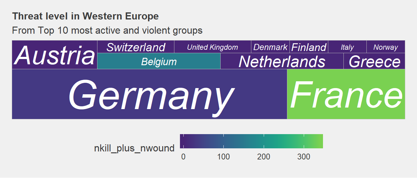
Figure 3.8: Threat level in Western Europe
The situation in Western Europe represents the opposite of what we have observed in Eastern Europe. Here we can see that terrorism from top ten groups is spread across most the countries. While France facing the biggest impact in terms of cumulative fatalities and injuries followed by Belgium, we can also see that Germany is facing the highest number of attacks.
| country | region | attack_count | nkill_plus_nwound |
|---|---|---|---|
| Austria | Western Europe | 5 | 0 |
| Belgium | Western Europe | 4 | 157 |
| Denmark | Western Europe | 1 | 0 |
| Finland | Western Europe | 1 | 1 |
| France | Western Europe | 12 | 338 |
| Germany | Western Europe | 28 | 30 |
| Greece | Western Europe | 2 | 0 |
| Italy | Western Europe | 1 | 0 |
| Netherlands | Western Europe | 4 | 4 |
| Norway | Western Europe | 1 | 1 |
| Switzerland | Western Europe | 2 | 0 |
| United Kingdom | Western Europe | 2 | 0 |
Based on threat level, we can identify Germany and France as major epicenters and Belgium as a minor epicenter in the Western Europe region. It should be noted that the threat level in Ukraine alone is almost 5 times higher than the threat level in the whole Western Europe region.
tmp1 <- tmp %>%
  filter(region %in% c("Middle East & North Africa",
                       "Sub-Saharan Africa", "South Asia"))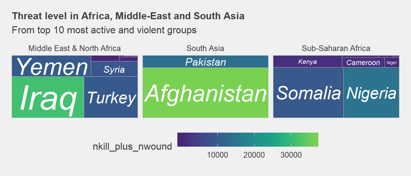
Figure 3.9: Threat level in Africa, Middle-East and South Asia
| country | region | attack_count | nkill_plus_nwound |
|---|---|---|---|
| Afghanistan | South Asia | 3199 | 36364 |
| Iraq | Middle East & North Africa | 1480 | 31169 |
| Nigeria | Sub-Saharan Africa | 746 | 14540 |
| Pakistan | South Asia | 783 | 13192 |
| Yemen | Middle East & North Africa | 825 | 9334 |
| Turkey | Middle East & North Africa | 1102 | 9259 |
| Somalia | Sub-Saharan Africa | 942 | 8963 |
| Syria | Middle East & North Africa | 352 | 8776 |
| Cameroon | Sub-Saharan Africa | 111 | 2170 |
| Kenya | Sub-Saharan Africa | 213 | 1771 |
| Niger | Sub-Saharan Africa | 39 | 859 |
| Saudi Arabia | Middle East & North Africa | 81 | 509 |
| Chad | Sub-Saharan Africa | 17 | 378 |
| Lebanon | Middle East & North Africa | 42 | 377 |
| Ethiopia | Sub-Saharan Africa | 4 | 102 |
| Jordan | Middle East & North Africa | 3 | 58 |
| Tunisia | Middle East & North Africa | 2 | 31 |
| Djibouti | Sub-Saharan Africa | 1 | 20 |
| Iran | Middle East & North Africa | 1 | 11 |
| Libya | Middle East & North Africa | 2 | 7 |
| Tanzania | Sub-Saharan Africa | 1 | 7 |
| Israel | Middle East & North Africa | 1 | 4 |
| Burkina Faso | Sub-Saharan Africa | 1 | 2 |
| Egypt | Middle East & North Africa | 1 | 2 |
| Uganda | Sub-Saharan Africa | 3 | 1 |
| West Bank and Gaza Strip | Middle East & North Africa | 2 | 1 |
From the plot and table above, we can see that all three regions are heavily impacted. While Afghanistan facing the largest impact in terms of fatalities and number of people injured followed by Iraq, we can also see that the spread in Southeast Asia is limited to Pakistan and Afghanistan only (similar to Eastern Europe).
In the case of Sub-Saharan Africa and the Middle East & North Africa region, we can see spread across many countries. We can also see many countries with a low number of attacks but the relatively large number of fatalities and injuries such as in Yemen, Niger, Nigeria, and Chad. In a comparison to other regions, the cumulative sum of a number of fatalities and injuries in Africa, Middle-East, and South Asia is more than 9,000 in each of the top five highly impacted countries.
To further identify the epicenters by each group, let us narrow down our analysis to the city level. For this analysis, I have set the threshold for a cumulative number of fatalities and injuries to 100 and have removed observations where the name of the city is unknown as shown in the code chunk below:
#------------------------------------------
#Epicenters at city level per group
#------------------------------------------
tmp <- df %>%
  filter(group_name %in% top10_groups) %>%
  replace_na(list(nkill = 0, nwound = 0)) %>%
  group_by(group_name, region, year, month) %>%
  filter(if_else(part_of_multiple_attacks == 1,
                 nkill == max(nkill) & nwound == max(nwound),
                 nkill == nkill & nwound == nwound)) %>%
  ungroup() %>%
  distinct(group_name, region, country, city, year, month,
           nkill, nwound, part_of_multiple_attacks) %>%
  group_by(city, group_name) %>%
  summarise(attack_count = n(),
            nkill_plus_nwound = sum(nkill + nwound)) %>%
  filter(nkill_plus_nwound >= 100 &
         city != "Unknown" &
         city != "unknown") %>%
as.data.frame()glimpse(tmp)Observations: 284
Variables: 4
$ city <chr> "Abu Adh Dhuhur", "Abu Ghraib", "Abuja", "Ad...
$ group_name <chr> "Al-Nusrah Front", "Islamic State of Iraq an...
$ attack_count <int> 4, 13, 9, 55, 21, 7, 45, 29, 24, 14, 8, 29, ...
$ nkill_plus_nwound <dbl> 132, 103, 444, 261, 346, 110, 164, 383, 592,...From the prepared data, we can see that 284 cities are impacted by the top 10 most active and violent groups. Next, we plot this data using treemap where the size/area represents a number of attacks and color represents the intensity of the cumulative sum of fatalities and injuries.
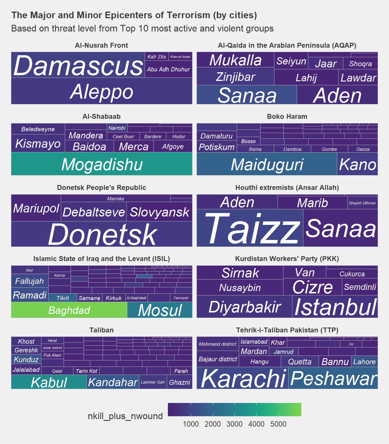
Figure 3.10: The Major and Minor Epicenters of Terrorism (by each group)
We can see distinct characteristic among the groups in terms of spread. For example, Al-Nusrah Front, Houthi Extremists and Donetsk People’s Republic groups have spread across 5 to 10 cities while having few major epicenters. Whereas ISIL, Taliban and Boko Haram groups have spread across many cities. In the case of ISIL, we can also see a relatively large number of fatalities and injuries with a low number of attacks in several cities.
To summarize, we identified the top 10 most lethal groups that are active between 2010 to 2016 and examined their characteristics behind attacks. We looked at the trend in the type of attack and a corresponding number of attacks over the period of time, which up to certain extent, indicates easy access to firearms and explosive devices either through illegal arms trade or through undisclosed support from powerful nation/s. We also examined pattern in target type, in which, 46.7% attacks were targeted at the Military and Police category and 27.3% attacks were intended toward civilians. Based on the threat level from the top ten groups, we examined the geographical spread and identified the hot spots where these groups are highly active.
Accessing GTD data: https://www.start.umd.edu/gtd/contact/↩
Searching and extracting data from the World Bank’s World Development Indicators. : https://cran.r-project.org/web/packages/WDI/WDI.pdf↩