Chapter 7 Predicting Class Probabilities
In our dataset, we have several categorical variables such as suicide attack, attack success, extended attack, part of multiple attacks etc with qualitative value i.e. Yes/ No (1 or 0). In the previous chapter, we have predicted a number of attacks and fatalities for Afghanistan, Iraq and SAHEL region. In this chapter, we choose data from all the countries that are impacted by top 10 most active and violent groups and make use of a cutting-edge LightGBM algorithm to predict the category of target variable which will be helpful to identify and understand the causal variables behind such attacks. This is a supervised machine learning approach, which means our dataset has labeled observations and the objective is to find a function that can be used to assign a class to unseen observations.
7.1 Evolution of Gradient Boosting Machines
In supervised learning, boosting is a commonly used machine learning algorithm due to its accuracy and efficiency. It is an ensemble model of decision trees where trees are grown sequentially i.e. each decision tree grown using the information from previously grown trees (James, Witten, Hastie, & Tibshirani, 2013). In other words, boosting overcomes the deficiencies in the decision trees by sequentially fitting the negative gradients to each new decision tree in the ensemble. Boosting method was further enhanced with optimization and as a result, Gradient Boosting Machine (GBM) came out a new approach to efficiently implement boosting method as proposed by the researcher (Friedman, 2001) in his paper “Greedy Function Approximation: A Gradient Boosting Machine”. GBM is also known as GBDT (Gradient Boosting Decision Tree). This approach has shown significant improvement in accuracy compared to traditional models. Although, this technique is quite effective but for every variable, boosting needs to scan all the data instances in order to estimate the information gain for all the possible splits. Eventually, this leads to increased computational complexities depending on a number of features and number of data instances (Ke et al., 2017).
To further explain this, finding optimal splits during the learning process is the most time-consuming part of traditional GBDT. The GBM package in R and XGBoost implements GBDT using pre-sorted algorithm to find optimal splits (T. Chen & Guestrin, 2016; Ridgeway, 2007). This approach requires scanning all the instances and then sorting them by feature gains. Another approach uses a histogram-based algorithm to bucket continuous variables into discrete bins. This approach focuses on constructing feature histograms through discrete bins during training process instead of finding splits based on sorted feature values (Ke et al., 2017). XGBoost supports both histogram-based and pre-sorted algorithm. Comparatively, the histogram-based approach is the most efficient in terms of training speed and RAM usage. From the year 2015, XGBoost has been widely recognized in many machine learning competitions (such as on Kaggle) as one of the best gradient boosting algorithm (T. Chen & Guestrin, 2016; Nielsen, 2016).
7.1.1 LightGBM
LightGBM is a fairly recent implementation of parallel GBDT process which uses histogram-based approach and offers significant improvement in training time and memory usage. The winning solutions from recent machine learning challenges on Kaggle and benchmarking of various GBM from the researcher (Pafka, 2018) indicate that LightGBM outperforms XGBoost and other traditional algorithms in terms of accuracy as well. LightGBM was developed by Microsoft researchers in October 2016 and it is an open-source library available in R and Python both.
7.1.2 The mechanism behind the improvised accuracy
The key difference between traditional algorithms and LightGBM algorithm is how trees are grown. Most decision tree learning algorithms controls the model complexity by depth and grow trees by level (depth-wise) as shown in the image below (image source12):
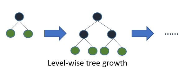
Figure 7.1: Level-wise tree growth in most GBDT algorithms
In contrast, the LightGBM algorithm uses a best-first approach and grows tree leaf-wise. As a result, the tree will choose the leaf with max delta loss to grow. According to (Microsoft Corporation, 2018), holding the leaf fixed, leaf-wise algorithms are able to achieve better accuracy i.e. lower loss compared to level-wise algorithms.
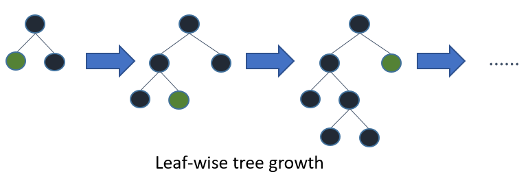
Figure 7.2: Leaf-wise tree growth in LightGBM algorithm
(image source13)
Researcher (Shi, 2007) further explains the phenomena behind tree growth in best-first and depth-first approach and suggests that most decision tree learners expand nodes in depth-first order whereas best-first tree learners expand the best node whose split achieves maximum reduction of impurity among all the nodes available for splitting. Although the resulting tree will be the same as a depth-wise tree, the difference is in the order in which it grown.
One of the key advantages of using LightGBM algorithm is that it offers good accuracy with label encoded categorical features instead of one hot encoded features. This eventually leads to faster training time. According to LightGBM documentation (Microsoft Corporation, 2018), the tree built on one-hot encoded features tends to be unbalanced and needs higher depth in order to achieve good accuracy in the case of categorical features with high-cardinality. LightGBM implements Exclusive Feature Bundling (EFB) technique, which is based on research by (D. Fisher, 1958) to find the optimal split over categories and often performs better than one-hot encoding.
One disadvantage of the leaf-wise approach is that it may cause over fitting when data is small. To overcome this issue, LightGBM includes the max_depth parameter to control model complexity, however, trees still grow leaf-wise even when max_depth is specified (Microsoft Corporation, 2018).
7.2 Data preparation
To understand the characteristics of the top 10 most active and violent terrorist groups, we filter the data and include all the countries that are impacted by this groups as shown in the code chunk below:
df_class <- df %>%
  filter(group_name %in% top10_groups) %>%
  select(suicide_attack, year, month, day, region, country,
         provstate, city, attack_type, target_type, weapon_type,
         target_nalty, group_name, crit1_pol_eco_rel_soc, crit2_publicize,
         crit3_os_intl_hmn_law, part_of_multiple_attacks,
         individual_attack, attack_success, extended,
         intl_logistical_attack, intl_ideological_attack,
         nkill, nwound, arms_export, arms_import, population,
         gdp_per_capita, refugee_asylum, refugee_origin,
         net_migration, n_peace_keepers, conflict_index) %>%
  replace_na(list(nkill = 0, nwound = 0)) %>%
  na.omit()
7.3 Overview of the target variable
For this analysis, I have selected suicide_attack as a target variable. According to GTD codebook, this variable is coded “Yes” in those cases where there is evidence that the perpetrator did not intend to escape from the attack alive.
| level | freq | perc | cumfreq | cumperc |
|---|---|---|---|---|
| No | 19319 | 0.887 | 19319 | 0.887 |
| Yes | 2461 | 0.113 | 21780 | 1.000 |
From the frequency table, we can see that 11.3% of incidents were observed as suicide attacks out of total 21,780 observations. Our objective is to train the classifier on training data (up to 2015) and correctly classify the instances of “Yes” in suicide attack variable in test data (the year 2016).
7.3.1 Dealing with class imbalance
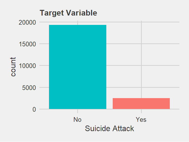
Figure 7.3: Overview of target variable: Suicide Attack
From the frequency table and the plot above, we can see that the target variable has a severe class imbalance where positive cases are present in only 11.3% observations. For the classification modeling, the class imbalance is a major issue and there are several techniques to deal with it such as down sampling, up sampling, SMOTE (Synthetic Minority Over-sampling Technique).
We use scale_pos_weight argument in the model building process which controls the weights of the positive observations. According to LightGBM documentation (Microsoft Corporation, 2018), default value for scale_pos_weight is 1.0 and it represents weight of positive class in binary classification task. We calculate this value as a number of negative samples/number of positive samples.
7.4 Feature engineering
Feature engineering is a process of creating representations of data that increase the effectiveness of a model (M. K. and K. Johnson, 2018). This is one of the most important aspects in machine learning that requires careful transformations and widening the feature space in order to improve the performance of the model. During the data cleaning process, we have already taken care of missing values and NAs. With regard to LightGBM model, the primary requirement is to have all the variables in numeric. As discussed earlier, LightGBM offers good accuracy with label encoded categorical features compared to the one-hot encoding method used in most algorithms. In this regard, we label encode all the categorical variables and specify them as a vector in model parameters. We also have numeric variables with extreme values such as arms_import, arms_export, nkill, nwound etc. For the modeling purpose, we use log transformation for such features. Last but not the least, we add frequency count features to widen the feature space. Frequency count features is a known technique in machine learning competitions to improve the accuracy of the model. An example of the feature with frequency is a number of attacks by the group, year and region. Use of frequency count features adds more context to data and will be helpful to improve the performance of the model.
#-------------------------------------------------------------
# Step 1: log transformation
#-------------------------------------------------------------
data <- df_class %>%
  mutate(nkill = log1p(nkill + 0.01),
         nwound= log1p(nwound + 0.01),
         arms_export = log1p(arms_export + 0.01),
         arms_import = log1p(arms_import + 0.01),
         population = log1p(population + 0.01))

#--------------------------------------------------------------
# Step 2: Add frequency count features
#--------------------------------------------------------------
data <- as.data.table(data)
data[, n_group_year:=.N,        by=list(group_name, year)]
data[, n_region_year:=.N,       by=list(region, year)]
data[, n_city_year:=.N,         by=list(city, year)]
data[, n_attack_year:=.N,       by=list(attack_type, year)]
data[, n_target_year:=.N,       by=list(target_type, year)]
data[, n_weapon_year:=.N,       by=list(weapon_type, year)]
data[, n_group_region_year:=.N, by=list(group_name, region, year)]
data[, n_group:=.N,             by=list(group_name)]
data[, n_provstate:=.N,         by=list(provstate)]
data[, n_city:=.N,              by=list(city)]
data <- as.data.frame(data)

#--------------------------------------------------------------
# Step 3: label encode categorical data (lightgbm requirement)
#--------------------------------------------------------------

features= names(data)
for (f in features) {
  if (class(data[[f]])=="character") {
    levels <- unique(c(data[[f]]))
    data[[f]] <- as.integer(factor(data[[f]], levels=levels))
  }
}

#--------------------------------------------------------------
# Step 4: Covert all the variable to numeric
#--------------------------------------------------------------
data[] <- lapply(data, as.numeric)
#str(data)
At this point, all of our variables are numeric and there are no missing values or NAs in this prepared data.
7.5 Validation strategy
In general, cross-validation is the widely used approach to estimate performance of the model. In this approach, training data is split into equal sized (k) folds. The model is then trained on k-1 folds and performance is measured on the remaining fold (M. K. and K. Johnson, 2018). However, this approach is not suitable for our data. To further explain this, the observations in our dataset are time-based so training the model on recent years (for example 2000- 2010) and evaluating the performance on previous years (for example 1980- 1990) would not be meaningful. To overcome this issue, we use a time-based split to evaluate the performance of our model. In other words, we use the observations in the year 2016 as the test set and the remaining observations as our training set.
This way we can be ensured that the model we have trained is capable of classifying target variable in current context. Following is the code used to implement validation strategy:
#--------------------------------------
# validation split
#--------------------------------------
train <- data %>% filter(year <= 2015)
test  <- data %>% filter(year == 2016)
The next stage of the process is to convert our data into lgb.Dataset format. During this process, we create a vector containing names of all our categorical variables and specify it while constructing lgb.Dataset as shown in the code below:
#--------------------------------------
# define all categorical features
#--------------------------------------
cat_vars <- df %>%
  select(year, month, day, region, country,
         provstate, city, attack_type, target_type, weapon_type,
         target_nalty, group_name, crit1_pol_eco_rel_soc, crit2_publicize,
         crit3_os_intl_hmn_law, part_of_multiple_attacks,
         individual_attack, attack_success, extended,
         intl_logistical_attack, intl_ideological_attack,
         conflict_index) %>%
  names()

#----------------------------------------------------------------------------
# construct lgb.Dataset, and specify target variable and categorical features
#----------------------------------------------------------------------------
dtrain = lgb.Dataset(
  data = as.matrix(train[, colnames(train) != "suicide_attack"]),
  label = train$suicide_attack,
  categorical_feature = cat_vars
  )

dtest = lgb.Dataset(
  data = as.matrix(test[, colnames(test) != "suicide_attack"]),
  label = test$suicide_attack,
  categorical_feature = cat_vars
  )
Notice that we have assigned labels separately to training and test data. To summarize the process, we will train the model on training data (dtrain), evaluate performance on test data (dtest).
7.6 Hyperparameter optimization
Hyperparameter tuning is a process of finding the optimal value for the chosen model parameter. According to (M. K. and K. Johnson, 2018), parameter tuning is an important aspect of modeling because they control the model complexity. And so that, it also affects any variance-base trade-off that can be made. There are several approaches for hyperparameter tuning such as Bayesian optimization, grid-search, and randomized search. For this analysis, we used random grid-search approach for hyperparameter optimization. In simple words, Randomized grid-search means we concentrate on the hyperparameter space that looks promising. This judgment often comes with the prior experience of working with similar data. Several researchers (Bergstra & Bengio, 2012; Bergstra, Bardenet, Bengio, & Kégl, 2011) have also supported the randomized grid-search approach and have claimed that random search is much more efficient than any other approaches for optimizing the parameters.
For this analysis, we choose number of leaves, max depth, bagging fraction, feature fraction and scale positive weight which are the most important parameters to control the complexity of the model. As shown in the code chunk below, first we define a grid by specifying parameter and iterate over a number of models in grids to find the optimal parameter values.
set.seed(84)
#--------------------------------------
# define grid in hyperparameter space
#--------------------------------------
grid <- expand.grid(
  num_leaves        = c(5,7,9),
  max_depth         = c(4,6),
  bagging_fraction  = c(0.7,0.8,0.9),
  feature_fraction  = c(0.7,0.8,0.9),
  scale_pos_weight  = c(4,7)
)

#--------------------------------------
# Iterate model over set grid
#--------------------------------------
model <- list()
perf <- numeric(nrow(grid))

for (i in 1:nrow(grid)) {
  # cat("Model ***", i , "*** of ", nrow(grid), "\n")
  model[[i]] <- lgb.train(
      list(objective         = "binary",
           metric            = "auc",
           learning_rate     = 0.01,
           num_leaves        = grid[i, "num_leaves"],
           max_depth         = grid[i, "max_depth"],
           bagging_fraction  = grid[i, "bagging_fraction"],
           feature_fraction  = grid[i, "feature_fraction"],
           scale_pos_weight  = grid[i, "scale_pos_weight"]),
      dtrain,
      valids = list(validation = dtest),
      nthread = 4,
      nrounds = 5,
      verbose= 0,
      early_stopping_rounds = 3
    )
  perf[i] <- max(unlist(model[[i]]$record_evals[["validation"]][["auc"]][["eval"]]))
  invisible(gc()) # free up memory after each model run
}
#--------------------------------------
#Extract results
#--------------------------------------
cat("Model ", which.max(perf), " is with max AUC: ", max(perf), sep = "","\n")Model 42 is with max AUC: 0.9538best_params = grid[which.max(perf), ]| num_leaves | max_depth | bagging_fraction | feature_fraction | scale_pos_weight | |
|---|---|---|---|---|---|
| 42 | 9 | 6 | 0.7 | 0.9 | 4 |
From the hyperparameter tuning, we have extracted the optimized values based on AUC. Next, we use these parameters in the model building process.
7.7 Modelling
# assign params from hyperparameter tuning result
params <- list(objective = "binary",
               metric = "auc",
               num_leaves = best_params$num_leaves,
               max_depth = best_params$max_depth,
               bagging_fraction = best_params$bagging_fraction,
               feature_fraction = best_params$feature_fraction,
               scale_pos_weight= best_params$scale_pos_weight,
               bagging_freq = 1,
               learning_rate = 0.01)

model <- lgb.train(params,
                   dtrain,
                   valids = list(validation = dtest),
                   nrounds = 1000,
                   early_stopping_rounds = 50,
                   eval_freq = 100)
[1]: validation's auc:0.937756
[101]: validation's auc:0.961098
[201]: validation's auc:0.962072
[301]: validation's auc:0.963493 7.7.1 Model evaluation
In order to evaluate the performance of our model on test data, we have used AUC metric which is commonly used in binary classification problem. From the trained model, we extract AUC score on test data from the best iteration with the code as shown below:
cat("Best iteration: ", model$best_iter, "\n")Best iteration: 288 cat("Validation AUC @ best iter: ",
max(unlist(model$record_evals[["validation"]][["auc"]][["eval"]])), "\n")Validation AUC @ best iter: 0.9636 To deal with overfitting, we have specified early stopping criteria which stops the model training if no improvement is observed within specified rounds. At the best iteration, our model achieves 96.36% accuracy on validation data. To further investigate the error rate, we use the confusion matrix.
7.7.2 Confusion Matrix
A confusion matrix is an another way to evaluate performance of binary classification model.
# get predictions on validation data
test_matrix <- as.matrix(test[, colnames(test) != "suicide_attack"])
test_preds = predict(model, data = test_matrix, n = model$best_iter)

confusionMatrix(
  data = as.factor(ifelse(test_preds > 0.5, 1, 0)),
  reference = as.factor(test$suicide_attack)
  )
Confusion Matrix and Statistics
Reference
Prediction 0 1
0 3339 91
1 249 582
Accuracy : 0.92
95% CI : (0.912, 0.928)
No Information Rate : 0.842
P-Value [Acc > NIR] : <0.0000000000000002
Kappa : 0.726
Mcnemar's Test P-Value : <0.0000000000000002
Sensitivity : 0.931
Specificity : 0.865
Pos Pred Value : 0.973
Neg Pred Value : 0.700
Prevalence : 0.842
Detection Rate : 0.784
Detection Prevalence : 0.805
Balanced Accuracy : 0.898
'Positive' Class : 0
The accuracy of 0.92 indicates that our model is 92% accurate. Out of all the metrics, the one we are most interested in is specificity. We want our classifier to predict the “Yes”/ “1” instances of suicide attack with higher accuracy. From the contingency table, we can see that our model has correctly predicted 582 out of 673 instances of “1”/ “Yes” in suicide attacks and achieves an accuracy of 86.5%.
7.7.3 Feature importance
# get feature importance
fi = lgb.importance(model, percentage = TRUE)| Feature | Gain | Cover | Frequency |
|---|---|---|---|
| weapon_type | 0.4447 | 0.2088 | 0.0773 |
| nkill | 0.1883 | 0.1298 | 0.1389 |
| provstate | 0.1285 | 0.2174 | 0.2370 |
| attack_type | 0.0781 | 0.1080 | 0.0616 |
| target_type | 0.0353 | 0.0618 | 0.0964 |
| nwound | 0.0291 | 0.0591 | 0.0820 |
| attack_success | 0.0229 | 0.0244 | 0.0464 |
| city | 0.0221 | 0.0979 | 0.0543 |
| day | 0.0110 | 0.0279 | 0.0699 |
| n_attack_year | 0.0069 | 0.0095 | 0.0195 |
| group_name | 0.0067 | 0.0081 | 0.0165 |
| n_peace_keepers | 0.0052 | 0.0049 | 0.0143 |
| refugee_origin | 0.0048 | 0.0048 | 0.0130 |
| target_nalty | 0.0033 | 0.0121 | 0.0156 |
| n_city_year | 0.0018 | 0.0019 | 0.0043 |
Gain is the most important measure for predictions and represents feature contribution to the model. This is calculated by comparing the contribution of each feature for each tree in the model. The Cover metric indicates a number of observations related to the particular feature. The Frequency measure is the percentage representing the relative number of times a particular feature occurs in the trees of the model. In simple words, it tells us how often the feature is used in the model (T. Chen, Tong, Benesty, & Tang, 2018; Pandya, 2018).
From the feature importance matrix, we can see that type of weapon contributes the most in terms of gain followed by number of people killed, province state, type of attack and type of target. In order to allow the model to decide whether an attack will be a suicide attack or not, these features are the most important compared to others.
7.8 Model interpretation
To further analyze the reasoning behind the model’s decision-making process, we randomly select one observation from test data and compare it with the predicted value based on features contribution. With the code chunk as shown below, we have extracted the predicted value from our trained model for the second observation in the test data.
cat(paste("predicted value from model: ", test_preds[[2]]))predicted value from model: 0.854690873381908The predicted value is 0.85 (i.e. > 0.5) which means our model indicates that the incident likely to be a suicide attack (i.e. “Yes” instance in suicide attack variable). Next, we use lgb.interpret function to compute feature contribution components of raw score prediction for this observation.
#extract interpretation for 2nd observation in (transformed) test data
test_matrix <- as.matrix(test[, colnames(test)])
tree_interpretation <- lgb.interprete(model, data = test_matrix, idxset = 2)
Figure 7.4: Model interpretation for 2nd observation
In the plot above, ten most important features (with higher contribution) are shown on the Y axis and their contribution value is on the X-axis. The negative value indicates contradiction and a positive value represents support. Our trained model has taken the decision to predict 0.85 for the second observation based on the contribution level of the above-mentioned features. Although nkill and weapon_type variables are one of most important features based on gain however their contribution toward prediction is negative. On the other hand, province, city, attack type and attack success features have a positive value which indicates support.
In our model, we have transformed the data to numeric. However, we can extract the raw test data (before transformation) and specific columns to compare the actual values with feature contribution plot above.
# extract raw test data
tmp_test <- df_class %>%
  filter(year == 2016) %>%
  select(suicide_attack, nkill, provstate, weapon_type,
         attack_type, city, attack_success, target_type,
         refugee_origin, n_peace_keepers)

# Extract second observation
tmp_test <- as.data.frame(t(tmp_test[2, ]))

# display result
knitr::kable(tmp_test, booktabs= TRUE,
             caption = "Actual values in 2nd observation in test set") %>%
kable_styling(latex_options = "HOLD_position", font_size = 12, full_width = F)| 2 | |
|---|---|
| suicide_attack | 1 |
| nkill | 3 |
| provstate | Kabul |
| weapon_type | Explosives/Bombs/Dynamite |
| attack_type | Bombing/Explosion |
| city | Kabul |
| attack_success | 1 |
| target_type | Business |
| refugee_origin | 2501410 |
| n_peace_keepers | 14 |
The predicted value from our model for the second observation is 0.85 and comparing it with actual value suggests that the incident was, in fact, a suicide attack as shown in the table above where the value is “1” in suicide attack variable. For this specific observation, our model suggests that Kabul as a city and provstate, Bombing/Explosion as attack type and attack being successful contributes positively toward prediction. In contrast, 3 fatalities, business as a target type and explosives as a weapon type contributes negatively to the prediction. Our trained model has correctly predicted 582 out of 673 instances of “1”/ “Yes” in suicide attacks and achieves an accuracy of 86.5% with this decision making process.