Chapter 4 Statistical Hypothesis Testing
In this chapter, first, we examine the strength of the relationship between two numerical variables using Pearson correlation coefficient. This way, we can get an idea of which variables have strong/weak and positive/negative correlation with each other. In the second part, we perform a hypothesis test between each of the top ten groups and the number of fatalities to see which groups represent similarity and differences. We use the data related to the top ten most active and violent groups only.
4.1 Data preparation
dfh <- df %>%
  filter(group_name %in% top10_groups) %>%  # filter data by top 10 groups
  replace_na(list(nkill = 0, nwound = 0))   # replace NAs

# Shorten lengthy group names
dfh$group_name[dfh$group_name == "Kurdistan Workers' Party (PKK)"] <- "PKK"
dfh$group_name[dfh$group_name == "Al-Qaida in the Arabian Peninsula (AQAP)"] <- "AQAP"
dfh$group_name[dfh$group_name == "Houthi extremists (Ansar Allah)"] <- "Houthi_Extrm"
dfh$group_name[dfh$group_name == "Tehrik-i-Taliban Pakistan (TTP)"] <- "TTP"
dfh$group_name[dfh$group_name == "Al-Nusrah Front"] <- "Al-Nusrah"
dfh$group_name[dfh$group_name == "Islamic State of Iraq and the Levant (ISIL)"] <-"ISIL"
dfh$group_name[dfh$group_name == "Donetsk People's Republic"] <- "Donetsk_PR"
4.2 Correlation test
We use pairwise complete observations method to compute correlation coefficients for each pair of numerical variables.
#Extract numeric variables
tmp <- dfh %>%
  select(intl_ideological_attack, intl_logistical_attack,
         part_of_multiple_attacks, n_peace_keepers, net_migration,
         refugee_asylum, refugee_origin, gdp_per_capita, arms_import,
         arms_export, conflict_index, population, extended,
         nwound, nkill, suicide_attack, attack_success)

# get the correlation matrix
m <- cor(tmp, use="pairwise.complete.obs")
# Get rid of all non significant correlations
ctest <- PairApply(tmp, symmetric=TRUE,
                   function(x, y) cor.test(x, y)$p.value)
m[ctest > 0.05] <- NA   # Replace p value > 0.05 with NAs
PlotWeb(m, lwd = abs(m[lower.tri(m)] * 10),
        main="Correlation Web Plot",
        cex.lab = 0.85, pt.bg = "#f2f2f2",
        args.legend = list(x = "bottomright", cex = 0.75, bty = "0",
                           title = "Correlation"))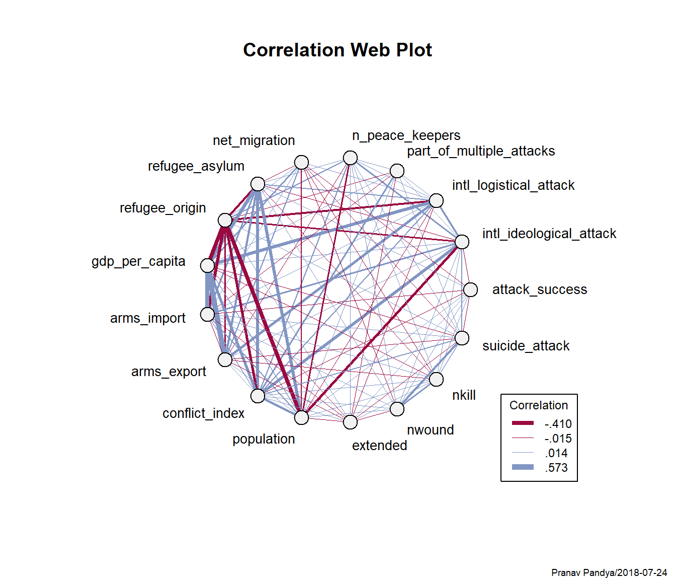
Figure 4.1: Correlation web plot
In the plot above, line width between the nodes is used in proportion to the correlation of two variables. To focus only on significant correlations, I have replaced observations with p-value more than 0.05 with NA. Legend on the bottom right represents correlation coefficient by line width and color depending on positive or negative linear relationship. The variables on the left-hand side of the plot are extracted from World Bank data (development indicators) and variables on the right-hand side are from GTD.
Specifically, we are more interested in the relationship to the variables on the right-hand side which will be used in time-series forecasting and classification modeling as the target variable. For example, a number of people wounded (nwound) variable has a positive linear relationship with a suicide attack. The conflict index variable shows a strong positive relationship with international ideological attacks and minor positive relationship with a part of multiple attacks. Overall, we can see that the majority of numerical variables shows a relationship with each other.
4.3 Hypothesis test: fatalities vs groups
The objective behind this hypothesis test is to determine whether or not means of the top 10 groups with respect to average fatalities are same. If at least one sample mean is different to others then we determine which pair of groups are different.
\[ \large \begin{aligned} {H_0 : } & \text{ The means of the different groups are the same} \\ &{(ISIL)} = {(Taliban)} = {(AQAP)} = {(PKK)} = \\ &{(Al-Shabaab)} = {(TTP)} = {(Boko Haram)} = \\ &{(Al-Nusrah)} = {(Donetsk_PR)} = {(Houthi_Extrm)} \\ \\ H_a: & \text{ At least one sample mean is not equal to the others} \end{aligned} \]
First, we use a box plot to examine distribution by quartiles for each group.
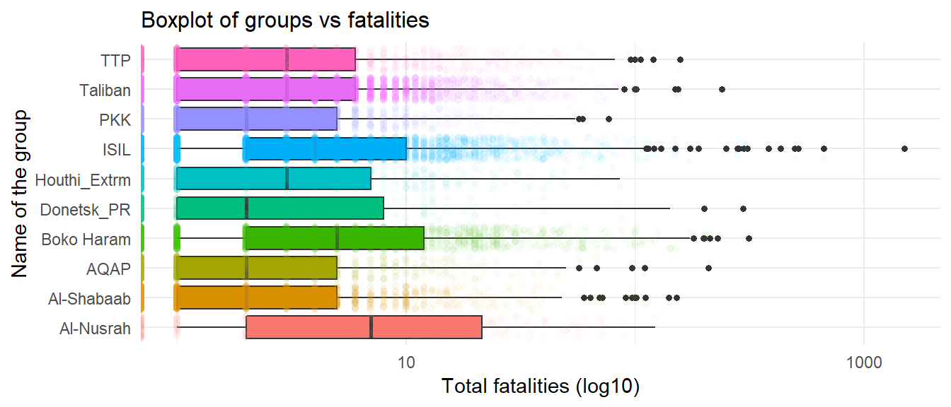
Figure 4.2: Boxplot: group vs fatalities
In statistical terms, we have some extreme outliers i.e. nkill ~ 1500 in ISIL group so X axis is log transformed for visualization purpose.
4.3.1 ANOVA test
The ANOVA model computes the residual variance and the variance between sample means in order to calculate the F-statistic. This is the first step to determine whether or not means are different in a pair of groups.
\[ \large \begin{aligned} F-statistic = & (S^2_{between}\ / S^2_{within}) \end{aligned} \]
#------------------------------------------
# Compute the analysis of variance (ANOVA)
#------------------------------------------
r.aov <- aov(nkill ~ group_name , data = dfh)

# display result
summary(r.aov)
Df Sum Sq Mean Sq F value Pr(>F)
group_name 9 111070 12341 40.7 <0.0000000000000002 ***
Residuals 21770 6597154 303
---
Signif. codes: 0 '***' 0.001 '**' 0.01 '*' 0.05 '.' 0.1 ' ' 1The model summary provides us F value and Pr(>F) corresponding to the p-value of the test. As we can see that the p-value is < 0.05, which means there are significant differences between the groups. In other words, we reject the null hypothesis. From this test, we identified that some of the group means are different however we don’t know which pair of groups have different means.
4.3.2 PostHoc test
PostHoc test is useful to determine where the differences occurred between groups. For this test, we use several different methods for the comparison purpose. This method can be classified as either conservative or liberal approach. Conservative methods are considered to be robust against committing Type I error as they use more stringent criterion for statistical significance. First, we run the PostHoc test by comparing results (p-value) from The Fisher LSD (Least Significant Different), Scheffe and Dunn’s (Bonferroni) test.
#------------------------------------------
# compare p-values for 3 methods
#------------------------------------------
posthoc1 <- as.data.frame(
  cbind(
    lsd= PostHocTest(
      r.aov, method="lsd")$group_name[,"pval"],     # The Fisher LSD
    scheffe= PostHocTest(
      r.aov, method="scheffe")$group_name[,"pval"], # Scheffe
    bonf=PostHocTest(
      r.aov, method="bonf")$group_name[,"pval"])    # Bonferroni
  )
posthoc1 <- rownames_to_column(posthoc1, var = "Pair of groups") %>%
  arrange(desc(scheffe))
|
|
The Fisher LSD (Least Significant Different) test is the most liberal in all the PostHoc tests whereas the Scheffe test is the most conservative and protects against Type I error. On the other hand, Dunn’s (Bonferroni) test is extremely conservative (Andri Signorell et mult. al., 2018). Out of all the possible combination of pairs (45), 16 pair of groups indicates p adj value > 0.9 based on the Scheffe test. In statistical terms, it means 16 pairs of groups as shown in the table above have non-significantly different means in a number of fatalities.
Next, we use Tukey HSD (Honestly Significant Difference) method which is the most common and preferred method.
#---------------------------------------
# PostHoc Test with Tukey HSD method
#---------------------------------------
#extract only p-values by setting conf.level to NA
hsd <- PostHocTest(r.aov, method = "hsd", conf.level=NA)
# convert to data frame and round off to 3 digits
hsd <- as.data.frame(do.call(rbind, hsd)) %>% round(3)| Al-Nusrah | Al-Shabaab | AQAP | Boko Haram | Donetsk_PR | Houthi_Extrm | ISIL | PKK | Taliban | |
|---|---|---|---|---|---|---|---|---|---|
| Al-Shabaab | 0.000 | NA | NA | NA | NA | NA | NA | NA | NA |
| AQAP | 0.000 | 0.981 | NA | NA | NA | NA | NA | NA | NA |
| Boko Haram | 0.783 | 0.000 | 0.000 | NA | NA | NA | NA | NA | NA |
| Donetsk_PR | 0.000 | 1.000 | 0.996 | 0.000 | NA | NA | NA | NA | NA |
| Houthi_Extrm | 0.000 | 1.000 | 1.000 | 0.000 | 1.000 | NA | NA | NA | NA |
| ISIL | 0.027 | 0.000 | 0.000 | 0.008 | 0.000 | 0.000 | NA | NA | NA |
| PKK | 0.000 | 0.990 | 0.687 | 0.000 | 1.000 | 0.992 | 0 | NA | NA |
| Taliban | 0.000 | 0.285 | 1.000 | 0.000 | 0.912 | 0.953 | 0 | 0.018 | NA |
| TTP | 0.000 | 0.073 | 0.916 | 0.000 | 0.457 | 0.499 | 0 | 0.007 | 0.879 |
4.3.3 Interpretation
The pairs of groups with adj p-value near or equals to 1 represents non-significantly different means in a number of fatalities such as Boko Haram - Al-Nusrah, Al-Qaida in Arabian Peninsula (AQAP)- Al-Shabaab, Houthi Extremist- PKK, Taliban- Tehrik-i-Taliban etc.
Similarly, a pair of groups with adjusted p-value near zero indicates significantly different means in a number of fatalities such as pairs of ISIL with all the remaining groups, Taliban - Al-Nusrah, PKK - Boko Haram, Donetsk_PR - Al-Nusrah etc.